
Audio Signal Classification System
Overview
As part of Speech Processing Course, this project implements an audio signal classification system that uses machine learning to classify audio signals into two distinct classes (e.g., “forward” and “backward”). The system captures audio signals, extracts relevant features, and applies multiple machine learning models to classify the signals. It demonstrates proficiency in audio signal processing, feature extraction, and machine learning model evaluation.
Spectrogram Analysis for Class Differentiation
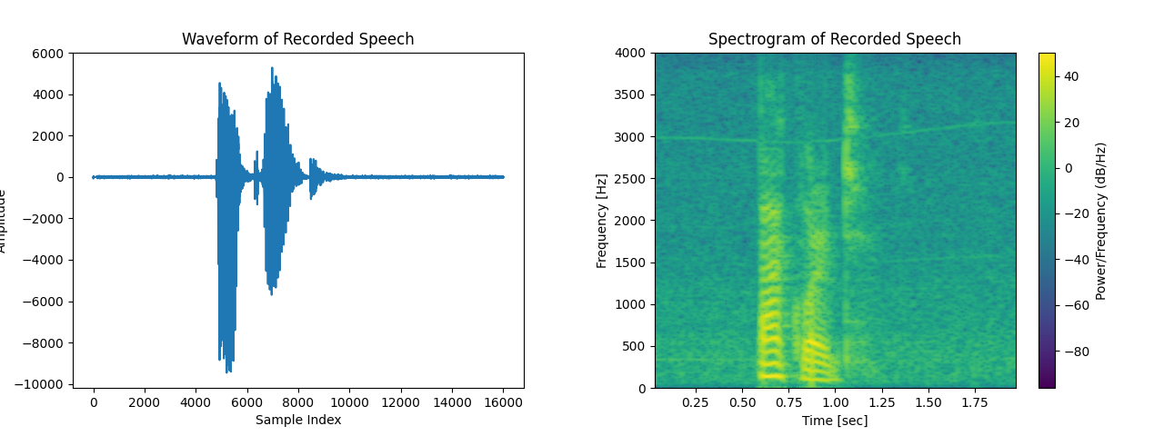
To gain deeper insight into the frequency domain characteristics of the two audio classes (“forward” and “backward”), spectrograms were generated. A spectrogram is a time-frequency representation of an audio signal, where the x-axis represents time, the y-axis represents frequency, and color intensity indicates the magnitude of the signal at a particular frequency.
Generating Spectrograms
The following code was used to generate and visualize the spectrograms:
f, t, Sxx = scipy.signal.spectrogram(mySpeech[:, 0], Fs, window=('kaiser', 5), nperseg=500, noverlap=475)
plt.pcolormesh(t, f, 10 * np.log10(Sxx), shading='gouraud')
Observations from Spectrograms
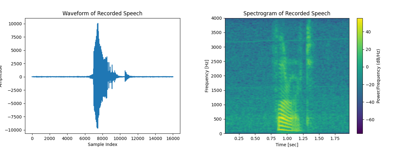
- Class 1 (Forward): The spectrogram shows dominant frequency components in the 0–1000 Hz range, with bursts of energy appearing at specific time intervals.
- Class 2 (Backward): The energy distribution is more spread out, with lower frequency components (below 1000 Hz) being more prominent.
These visual differences in frequency patterns suggest that feature extraction techniques based on frequency-domain analysis (e.g., Welch PSD, Mel-Frequency Cepstral Coefficients) can be effective for classification.
Key Features
- Audio Signal Capture: Records audio signals using a microphone with a sampling rate of 8000 Hz.
- Feature Extraction: Extracts 28 features from each audio signal using the Welch power spectral density (PSD) method.
- Data Preprocessing: Normalizes the data using
StandardScalerorMinMaxScalerand applies Principal Component Analysis (PCA) for dimensionality reduction. - Multiple Classifiers: Implements and evaluates 7 different machine learning models:
- Perceptron
- Feedforward Neural Network (Dense)
- Feedforward Neural Network (MLP)
- Support Vector Machine (SVM) with RBF, Polynomial, and Linear kernels
- K-Nearest Neighbors (KNN)
- Naive Bayes Classifier
- Parzen Window Estimator
- Model Evaluation: Evaluates each model using confusion matrices and accuracy scores.
Principal Component Analysis (PCA) and Feature Selection
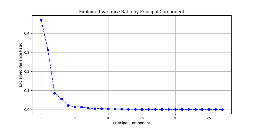
To improve classification performance and reduce computational complexity, Principal Component Analysis (PCA) was applied. PCA helps in dimensionality reduction by transforming the original feature space into a set of orthogonal principal components that retain most of the variance in the data.
The Cumulative Explained Variance Ratio was plotted to determine the number of principal components required to retain 90% of the variance. This ensures that the most significant features are preserved while eliminating redundant information.
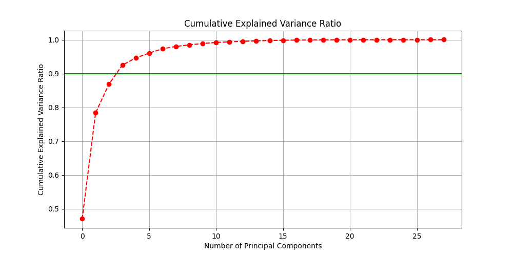
The green horizontal line at 0.90 (90%) marks the threshold for retaining information. The red curve shows the cumulative variance explained as the number of components increases. The point where this curve crosses 90% indicates the optimal number of components to select.
This ensures that only the most informative features are kept, improving model efficiency without sacrificing accuracy.
Technical Details
Workflow
- Audio Signal Capture:
- Records audio signals for 1.2 seconds using the
sounddevicelibrary. - Reshapes the signal and computes the Welch PSD to extract frequency-domain features.
- Records audio signals for 1.2 seconds using the
- Feature Extraction:
- Extracts 28 features from each signal using a custom
ext_paramfunction. - Stores features in a feature matrix
Xand labels in a target vectory.
- Extracts 28 features from each signal using a custom
- Data Preprocessing:
- Normalizes the data using
StandardScalerorMinMaxScaler. - Applies PCA to reduce dimensionality while retaining 90% of the variance.
- Normalizes the data using
- Model Training and Evaluation:
- Splits the data into training (70%) and testing (30%) sets.
- Trains and evaluates 7 machine learning models:
# Example: Perceptron
clf = Perceptron(tol=1e-15, eta0=0.001, max_iter=10000)
clf.fit(X_train, y_train)
predictions = clf.predict(X_test)
print('Confusion Matrix (Perceptron):\n', confusion_matrix(y_test, predictions))
print('Accuracy (Perceptron):', clf.score(X_test, y_test))
Performance Metrics
| Model | Accuracy | Confusion Matrix |
|---|---|---|
| Perceptron | 66% | [[5, 1], [3, 3]] |
| FF Neural Network | 88% | [[5, 1], [1, 5]] |
| FF MLP | 83% | [[5, 1], [1, 5]] |
| SVM (RBF Kernel) | 92% | [[6, 0], [1, 5]] |
| SVM (Poly Kernel) | 83% | [[5, 1], [1, 5]] |
| SVM (Linear Kernel) | 75% | [[5, 1], [2, 4]] |
| KNN | 87% | [[6, 0], [2, 4]] |
| Naive Bayes | 84% | [[5, 1], [1, 5]] |
| Parzen Window | 92% | [[6, 0], [1, 5]] |
Impact & Applications
This system demonstrates the ability to classify audio signals using machine learning, with applications in:
- Voice Command Recognition
- Sound Event Detection
- Biometric Authentication